Inspecting Demographics and Payment Patterns to Predict Credit Card Default Probability
Association:
iSchool, University of Toronto
Duration:
1.5 months
Data Science
Machine Learning
Python

For the final project in INF1340-Programming for Data Science, we worked on analyzing and predicting the default possibility of credit card owners.
Credit card debt and delinquency have always been one of the biggest pain points in the banking industry, implying socioeconomic and financial risks for both consumers and the servicing organizations. For consumers, delinquency can lead to a cycle of financial hardship, reduced access to credit, and long-term damage to creditworthiness. For financial institutions, high default rates increase operational risk, reduce profitability, and may necessitate stricter lending policies, which could limit access to credit for potential customers.
This study explores patterns and predictors of credit card default using a dataset that includes demographic, behavioral, and transactional variables. By employing descriptive and diagnostic analytics, such as pivot tables and statistical tests, and predictive modeling techniques, such as logistic regression and machine learning methods, the analysis identifies key factors contributing to default risk.
Diagnostic Analytics
After necessary data cleaning and descriptive analytics, we used diagnostic analytics to explore the potential relationships between variables, especially in relation to the target variable 'Default.'
# Visualize correlation with Heatmap
def correlation_matrix(df):
  numerical_df = df.select_dtypes(include=np.number)
  plt.figure(figsize=(16, 14))
  sns.heatmap(numerical_df.corr(), annot=True, cmap='coolwarm')
  plt.title('Correlation Heatmap')
  plt.show()
  return numerical_df.corr()

correlation_matrix(credit_data)

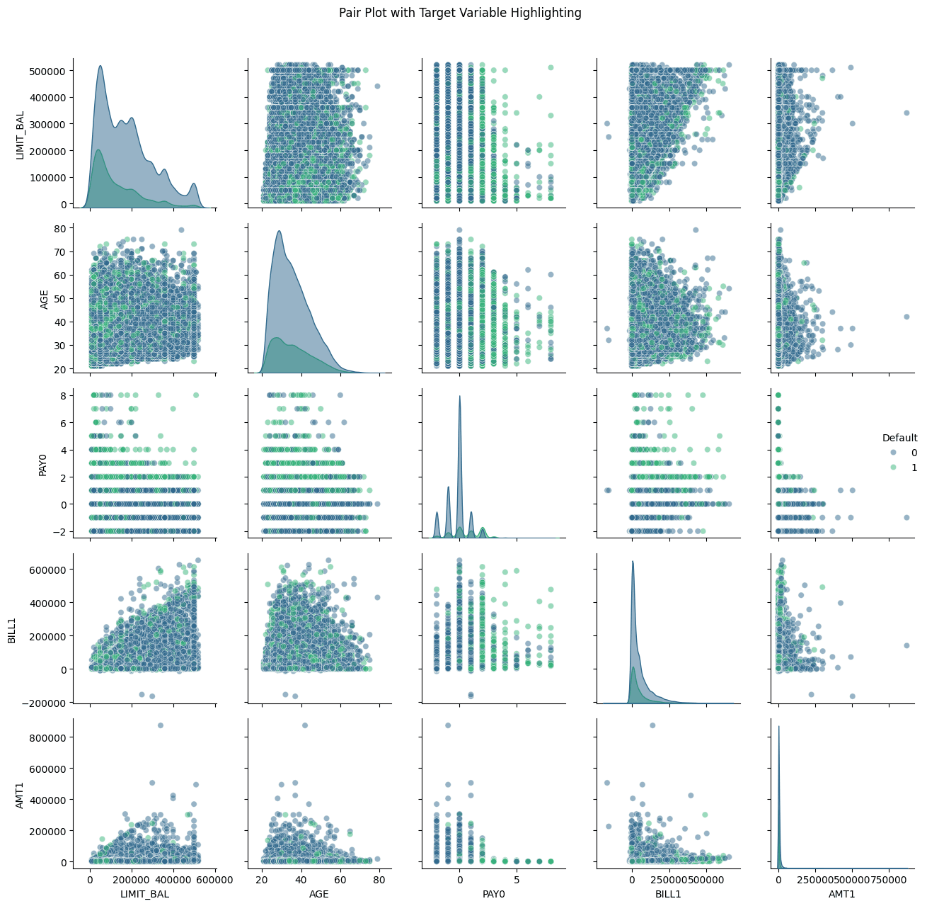
# Visualization for multivariate analysis
def multivariate_analysis(df):
  # Pair Plot with Hue based on Target Variable
  plt.figure(figsize=(15,10))
  subset_columns = ['LIMIT_BAL', 'AGE', 'PAY0', 'BILL1', 'AMT1', 'Default']
  g = sns.pairplot(df[subset_columns], hue='Default',
                     plot_kws={'alpha': 0.5},
                     diag_kws={'alpha': 0.5},
                     palette='viridis')
  g.fig.suptitle('Pair Plot with Target Variable Highlighting', y=1.02)
  plt.tight_layout()
  plt.show()

  # Parallel Coordinates Plot using Plotly
  def normalize_column(series):
        return (series - series.min()) / (series.max() - series.min())

  # Select columns for parallel coordinates
  parallel_cols = ['LIMIT_BAL', 'AGE', 'PAY0', 'BILL1', 'AMT1', 'Default']
  df_normalized = df[parallel_cols].copy()

  # Normalize numeric columns
  for col in parallel_cols[:-1]:  # Exclude target variable
      df_normalized[col] = normalize_column(df_normalized[col])

  # Create Parallel Coordinates Plot
  fig = px.parallel_coordinates(
        df_normalized,
        color='Default',
        title='Parallel Coordinates Plot',
        color_continuous_scale=px.colors.sequential.Viridis
  )
  fig.show()

  # Box Plots for Categorical Variables
  categorical_columns = ['SEX', 'EDUCATION', 'MARRIAGE']
  plt.figure(figsize=(15,5))

  for i, var in enumerate(categorical_columns, 1):
        plt.subplot(1, 3, i)
        sns.boxplot(x=var, y='LIMIT_BAL', hue='Default',
                    data=df, palette='Set2')
        plt.title(f'{var} vs Limit Balance by Default Status')
        plt.xticks(rotation=45)

  plt.tight_layout()
  plt.show()

multivariate_analysis(credit_data)


# Logistic regression analysis
def logistic_regression(df):

  # Select features and target variable
  X = X = df.drop(labels=['Default','AGE_GROUP'], axis=1)
  y = df['Default']

  # Split data into training and test sets
  X_train, X_test, y_train, y_test = train_test_split(X, y, test_size=0.3, random_state=42)

  # Logistic regression using statsmodels for detailed summary
  X_train_const = sm.add_constant(X_train)  # Adding constant for intercept
  logit_model = sm.Logit(y_train, X_train_const)
  result = logit_model.fit()

  # Display the summary to interpret coefficients and p-values
  print(result.summary())

logistic_regression(credit_data)

Logit Regression Results
==============================================================================
Dep. Variable:                Default   No. Observations:                20858
Model:                          Logit   Df Residuals:                    20834
Method:                           MLE   Df Model:                           23
Date:                Tue, 03 Dec 2024   Pseudo R-squ.:                  0.1253
Time:                        21:44:36   Log-Likelihood:                -9613.9
converged:                       True   LL-Null:                       -10991.
Covariance Type:            nonrobust   LLR p-value:                     0.000
==============================================================================
                 coef    std err          z      P>|z|      [0.025      0.975]
------------------------------------------------------------------------------
const         -0.6448      0.144     -4.473      0.000      -0.927      -0.362
LIMIT_BAL  -7.085e-07   1.93e-07     -3.663      0.000   -1.09e-06   -3.29e-07
SEX           -0.1047      0.037     -2.830      0.005      -0.177      -0.032
EDUCATION     -0.0685      0.026     -2.586      0.010      -0.120      -0.017
MARRIAGE      -0.1851      0.038     -4.818      0.000      -0.260      -0.110
AGE            0.0054      0.002      2.524      0.012       0.001       0.010
PAY0           0.5908      0.021     27.797      0.000       0.549       0.632
PAY2           0.0832      0.024      3.427      0.001       0.036       0.131
PAY3           0.0560      0.027      2.056      0.040       0.003       0.109
PAY4           0.0511      0.030      1.696      0.090      -0.008       0.110
PAY5           0.0378      0.033      1.162      0.245      -0.026       0.102
PAY6          -0.0057      0.027     -0.213      0.832      -0.058       0.047
BILL1      -5.429e-06   1.39e-06     -3.918      0.000   -8.15e-06   -2.71e-06
BILL2       1.943e-06   1.85e-06      1.048      0.295   -1.69e-06    5.58e-06
BILL3        4.98e-07   1.68e-06      0.297      0.766   -2.79e-06    3.78e-06
BILL4      -1.174e-06   1.75e-06     -0.671      0.502    -4.6e-06    2.26e-06
BILL5       2.552e-06   1.97e-06      1.297      0.195   -1.31e-06    6.41e-06
BILL6       5.432e-07   1.47e-06      0.370      0.712   -2.34e-06    3.42e-06
AMT1       -1.216e-05   2.66e-06     -4.569      0.000   -1.74e-05   -6.95e-06
AMT2        -8.75e-06   2.46e-06     -3.552      0.000   -1.36e-05   -3.92e-06
AMT3       -5.074e-06    2.3e-06     -2.202      0.028   -9.59e-06   -5.59e-07
AMT4       -5.096e-06   2.19e-06     -2.327      0.020   -9.39e-06   -8.04e-07
AMT5       -3.515e-06   2.18e-06     -1.610      0.107   -7.79e-06    7.63e-07
AMT6       -1.779e-06   1.54e-06     -1.156      0.248    -4.8e-06    1.24e-06
Regarding the logistic regression, pseudo R-squared of 0.1253 indicates that about 12.53% of the variance in the dependent variable (Default) is explained by the model. The log-likelihood ratio (LLR) p-value is smaller than 0, which suggests the model is statistically significant overall. While pseudo R-squared values in logistic regression are typically lower than R-squared in linear regression, 12.53% suggests a moderate but not particularly strong fit.
Looking at the coefficients, p-values, and confidence intervals, the predictor’s impact on the likelihood of default is interpreted below:
LIMIT_BAL: The negative coefficient indicates that higher credit limits are associated with a lower likelihood of default. The coefficient is statistically significant (p < 0.05), but the effect size is small, suggesting that LIMIT_BAL alone may not be a strong predictor.
SEX, EDUCATION, MARRIAGE: These demographic variables are statistically significant, with p-values below 0.05. The signs of the coefficients suggest:
Male (coded as 1): Associated with a slightly lower likelihood of default.
Higher Education: Associated with a increased probability of default. Compared to 'Graduate School', having a 'High School' education is associated with a decrease in the log-odds of default by 0.1006.
Marital Status: The negative coefficient suggests that being married may reduce the likelihood of default.
AGE: Positively associated with default probability, meaning older age is associated with higher odds of default. Although significant, the small coefficient implies age alone has a limited effect on default likelihood.
Repayment History (PAY0 to PAY6): These are among the most influential predictors, as seen from large, positive coefficients for PAY0 and smaller yet significant coefficients for PAY2 and PAY3. The significance and positive signs indicate that higher values (i.e., delayed payments) increase the probability of default.
BILL1, BILL2, etc., and AMT1, AMT2, etc.: Many of these billing and payment amount features are statistically significant but with small coefficients, implying limited impact on default likelihood. Some values like BILL2 and AMT6 are not significant, meaning they don’t seem to add predictive value for default in this model.
Predictive Analytics
We used three different machine learning models for this dataset: Decision Tree, Logistic Regression, and Naive Bayes.
# Decision Tree
def decision_tree(df):

  # Select features and target variable
  X = df.drop(labels=['Default', 'AGE_GROUP'], axis=1)
  y = df['Default']

  # Train-test split
  X_train, X_test, y_train, y_test = train_test_split(X, y, test_size=0.3, random_state=42)

  # Train a basic Decision Tree
  clf = DecisionTreeClassifier(criterion='entropy', random_state=42)
  clf.fit(X_train, y_train)

  # Predict on test data and measure accuracy
  y_pred = clf.predict(X_test)
  accuracy = accuracy_score(y_test, y_pred)
  print(f'Basic Decision Tree Accuracy: {accuracy:.2f}')
  print(classification_report(y_test, y_pred))

  # Experiment with different tree depths
  depths = [3, 5, 10, None]
  accuracies = []
  for depth in depths:
    clf = DecisionTreeClassifier(criterion='entropy', max_depth=depth, random_state=42)
    clf.fit(X_train, y_train)
    y_pred = clf.predict(X_test)
    acc = accuracy_score(y_test, y_pred)
    accuracies.append(acc)
    print(f'Depth: {depth}, Accuracy: {acc:.2f}')

  # Plot accuracies vs. tree depths
  plt.figure(figsize=(10, 6))
  plt.plot([str(d) for d in depths], accuracies, marker='o')
  plt.title('Decision Tree Accuracy vs. Depth')
  plt.xlabel('Tree Depth')
  plt.ylabel('Accuracy')
  plt.show()

  # Visualize the decision tree
  plt.figure(figsize=(20, 10))
  tree.plot_tree(clf, feature_names=X.columns, class_names=['Yes', 'No'], filled=True)
  plt.title('Decision Tree Visualization')
  plt.show()

decision_tree(credit_data)

# Decision Tree Entropy
def decision_tree_entropy(df):
  from sklearn.model_selection import train_test_split
  from sklearn.tree import DecisionTreeClassifier
  from sklearn.metrics import accuracy_score, classification_report
  from sklearn import tree

  # Select features and target variable
  X = df.drop(labels=['Default', 'AGE_GROUP'], axis=1)
  y = df['Default']

  # Train-test split
  X_train, X_test, y_train, y_test = train_test_split(X, y, test_size=0.3, random_state=42)

  # Train a Decision Tree classifier using Information Gain (entropy)
  clf = DecisionTreeClassifier(criterion='entropy', random_state=42)
  clf.fit(X_train, y_train)

  # Extract feature importances (Information Gain) from the model
  information_gain = clf.feature_importances_

  # Create a DataFrame to display feature names and their Information Gain
  feature_importance_df = pd.DataFrame({
      'Feature': X.columns,
      'Information Gain': information_gain
  }).sort_values(by='Information Gain', ascending=False)

  # Display the DataFrame
  print(feature_importance_df)

  # Plot the Information Gain for each feature
  plt.figure(figsize=(12, 8))
  plt.barh(feature_importance_df['Feature'], feature_importance_df['Information Gain'], color='skyblue')
  plt.xlabel('Information Gain')
  plt.ylabel('Feature')
  plt.title('Information Gain for Each Attribute')
  plt.gca().invert_yaxis()
  plt.show()

decision_tree_entropy(credit_data)

Basic Decision Tree Accuracy: 0.72
              precision    recall  f1-score   support

           0       0.82      0.82      0.82      6918
           1       0.38      0.39      0.39      2022

    accuracy                           0.72      8940
   macro avg       0.60      0.60      0.60      8940
weighted avg       0.72      0.72      0.72      8940

Depth: 3, Accuracy: 0.82
Depth: 5, Accuracy: 0.81
Depth: 10, Accuracy: 0.80
Depth: None, Accuracy: 0.72


# Naıve Bayesian Classifiers
def naive_bayes(df):

    # Select features and target variable
    X = df.drop(labels=['Default'], axis=1)
    y = df['Default']

    # Train-test split
    X_train, X_test, y_train, y_test = train_test_split(X, y, test_size=0.3, random_state=42)

    # Scale the features
    scaler = StandardScaler()
    X_train_scaled = scaler.fit_transform(X_train)
    X_test_scaled = scaler.transform(X_test)

    # Model setup
    model = GaussianNB()
    model.fit(X_train_scaled, y_train)

    # Make predictions
    y_pred = model.predict(X_test_scaled)

    # Calculate metrics
    accuracy = accuracy_score(y_test, y_pred)
    report = classification_report(y_test, y_pred)
    conf_matrix = confusion_matrix(y_test, y_pred)

    # Print results
    print("\nNaive Bayesian Results:")
    print(f"Accuracy: {accuracy:.4f}")
    print("\nClassification Report:")
    print(report)

    # Plot confusion matrix
    plt.figure(figsize=(8, 6))
    sns.heatmap(conf_matrix, annot=True, fmt='d', cmap='Blues')
    plt.title('Confusion Matrix - Naıve Bayesian')
    plt.ylabel('True Label')
    plt.xlabel('Predicted Label')
    plt.show()

    return {
        "model": model,
        "accuracy": accuracy,
        "classification_report": report,
        "confusion_matrix": conf_matrix,
    }

results = naive_bayes(credit_data)

Naive Bayesian Results:
Accuracy: 0.7506

Classification Report:
              precision    recall  f1-score   support

           0       0.87      0.80      0.83      6918
           1       0.46      0.58      0.51      2022

    accuracy                           0.75      8940
   macro avg       0.66      0.69      0.67      8940
weighted avg       0.77      0.75

Overall, Naive Bayes (0.75) performs worse than both the linear regression (0.80) and decision tree models (up to 0.82). This lower accuracy compared to previous models suggests that Naive Bayes may not be the best choice for this dataset, especially given the complexity of relationships in financial data. Naive Bayes assumes feature independence, which might not hold for this dataset (e.g., financial metrics like billing amounts and payments are likely correlated). Naive Bayes achieves the highest recall for class 1 (0.58), indicating it is better at identifying defaults compared to the decision tree (0.39) and linear regression (0.24), but its precision for class 1 (0.46) is only slightly better than the decision tree (0.38) and worse than linear regression (0.70).
Conclusion
Key findings include:
Model-wise, the most important feature in predicting default status is PAY0–the most recent credit card payment status.
Younger age groups show higher default rates, likely reflecting financial inexperience or limited income.
Higher education levels are strongly associated with higher credit limits and might reduce the likelihood of default but their influence on default prediction is limited.
All models faced challenges due to the class imbalance (non-defaults significantly outnumber defaults).
This project demonstrates the trade-offs between different models in handling imbalanced datasets for credit default prediction. While logistic regression and decision trees excel in overall accuracy, Naive Bayes offers superior recall for defaults, which may align better with business goals focused on identifying risky customers. Further optimization through feature engineering, resampling, and advanced modeling techniques can enhance performance and address class imbalance effectively.
Other Projects


© 2026. All rights Reserved.
© 2026. All rights Reserved.